Adam wrote and asked for a discussion of xG. I’m so happy about this suggestion that I’m actually going to do two posts on the topic. In this post we’ll look at the xG for a single shot on goal; in a subsequent post we’ll discuss the xG for a passage of play and for an entire game.
xG stands for expected goals, and it’s famous enough now that it’s used almost routinely on Match of the Day. But what is it, why is it used, how is it calculated and is it all it’s cracked up to be?
It’s well-understood these days when trying to assess how well a team has performed in a game, that because goals themselves are so rare, it’s better to go beyond the final result and look at the match in greater statistical detail.
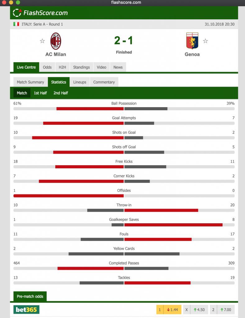
For example, this screenshot shows the main statistics for the recent game between Milan and Genoa, as provided by Flashscore. Milan won 2-1, but it’s clear from the data here that they also dominated the game in terms of possession and goal attempts. So, on the basis of this information alone, the result seems fair.
Actually, Milan’s winner came in injury time, and if they hadn’t got that goal, again on the basis of the above statistics, you’d probably argue that they would have been unlucky not to have won. In that case the data given here in terms of shots and possession would have given a fairer impression of the way the match played out than just the final result.
But even these statistics can be misleading: maybe most of Milan’s goal attempts were difficult, and unlikely to lead to goals, whereas Genoa’s fewer attempts were absolute sitters that they would score 9 times out of 10. If that were the case, you might conclude instead that Genoa were unlucky to lose. xG – or expected goals – is an attempt to take into account not just the number of chances a team creates, but also the difficulty of those chances.
The xG for a single attempt at goal is an estimate of the probability that, given the circumstances of a shot – the position of the ball, whether the shot is kicked or a header, whether the shot follows a dribble or not, and other relevant information – it is converted into a goal.
This short video from OPTA gives a pretty simple summary.
So how is xG calculated in practice? Let’s take a simple example. Suppose a player is 5 metres away from goal with an open net. Looking back through a database of many games, we might find (say) 1000 events of an almost identical type, and on 850 of those occasions a goal was scored. In that case the xG would be estimated as 850/1000 = 0.85. But breaking things down further, it might be that 900 of the 1000 events were kicked shots, while 100 were headers; and the number of goals scored respectively from these events were 800 and 50. We’d then calculate the xG for this event as 800/900 = 0.89 for a kicked shot, but 50/100 = 0.5 for a header.
But there are some complications. First, there are unlikely to be many events in the database corresponding to exactly the same situation (5 metres away with an open goal). Second, we might want to take other factors into account: scoring rates from the same position are likely to be different in different competitions, for example, or the scoring rate might depend on whether the shot follows a dribble by the same player. This means that simple calculations of the type described above aren’t feasible. Instead, a variation of standard regression – logistic regression – is used. This sounds fancy, but it’s really just a statistical algorithm for finding the best formula to convert the available variables (ball position, shot type etc.) into the probability of a goal.
So in the end, xG is calculated via a formula that takes a bunch of information at the time of a shot – ball position, type of shot etc. etc. – and converts it into a probability that the shot results in a goal. You can see what xG looks like using this simple app.
Actually, there are 2 alternative versions of xG here, that you can switch between in the first dialog box. For both versions, the xG will vary according to whether the shot is a kick or a header. For the second version the xG also depends on whether the shot is assisted by a cross, or preceded by a dribble: you select these options with the remaining dialog boxes. In either case, with the options selected, clicking on the graphic of the pitch will return the value of xG according to the chosen model. Naturally, as you get closer to the goal and with a more favourable angle the xG increases.
One point to note about xG is that there is no allowance for actual players or teams. In the OPTA version there is a factor that distinguishes between competitions – presumably since players are generally better at converting chances in some competitions than others – but the calculation of xG is identical for all players and teams in a competition. Loosely speaking, xG is the probability a shot leads to a goal by an average player who finds themselves in that position in that competition. So the actual xG, which is never calculated, might be higher if it’s a top striker from one of the best teams, but lower if it’s a defender who happened to stray into that position. And in exactly the same way, there is no allowance in the calculation of xG for the quality of the opposition: xG averages over all players, both in attack and defence.
It follows from all this discussion that there’s a subtle difference between xG and the simpler statistics of the kind provided by Flashscore. In the latter case, as with goals scored, the statistics are pure counts of different event types. Apart from definitions of what is a ‘shot on goal’, for example, two different observers would provide exactly the same data. xG is different: two different observers are likely to agree on the status of an event – a shot on an open goal from the corner of the goal area, for example – but they may disagree on the probability of such an event generating a goal. Even the two versions in the simple app above gave different values of xG, and OPTA would give a different value again. So xG is a radically different type of statistic; it relies on a statistical model for converting situational data into probabilities of goals being scored, and different providers may use different models.
We’ll save discussion about the calculation of xG for a whole match or for an individual player in a whole match for a subsequent post. But let me leave you with this article from the BBC. The first part is a summary of what I’ve written here – maybe it’s even a better summary than mine. And the second part touches on issues that I’ll discuss in a subsequent post. But half way down there’s a quiz in which five separate actions are shown and you’re invited to guess the value of xG for each. See if you can beat my score of 2/5.
Incidentally, why do we use the term ‘expected goals’ if xG is a probability? Well, let’s consider the simpler experiment of tossing a coin. Assuming it’s a fair coin, the probability of getting a head is 0.5. In (say) 1000 tosses of the coin, on average I’d get 500 heads. That’s 0.5 heads per toss, so as well as being the probability of a head, 0.5 is also the number of heads we expect to get (on average) when we toss a single coin. xH if you like. And the same argument would work for a biased coin that has probability 0.6 of coming up heads: xH = 0.6. And exactly the same argument works for goals: if xG is the probability of a certain type of shot becoming a goal, it’s also the expected goals we’d expect, per event, from events of that type.
And finally… if there are any other statistical topics that you’d like me to discuss in this blog, whether related to sports or not, please do write and let me know.