Hello Wimbledon and happy birthday to the longest tennis match in history. Played between John Isner and Nicolas Mahut, this Wimbledon first round mens’ single’s match started on 22 June, 2010 and finished 2 days later on 24 June. The total playing time was 11 hours, 5 minutes, making it the longest professional tennis match in history, both in terms of duration and games played. Not for no reason did it come to be called ‘the endless match’.
Under current tie-break rules, an event of this type couldn’t occur, but at the time of the match any 5th set at Wimbledon that reached 6 games all was played without tiebreaks until one of the players obtained a two-game advantage. Remarkably, this led to a situation where the final set score of the Isner-Mahut match was 70 games to 68 in favour of John Isner. That set alone lasted 8 hours and 11 minutes.
With all that in mind, think about the following question.
Question:
What was the probability that the final set in the Isner-Mahut match would finish, as it did, 70 games to 68?
Make a calculated guess and then scroll down for some discussion.
|
|
|
|
|
|
|
|
|
|
|
|
|
|
|
|
Perhaps more than any other sport, tennis invites analysis via simple mathematical, statistical and probabilistic arguments. If, for example, we make the following assumptions:
- The player serving wins each point with probability p;
- All points are independent of all others (so the outcome of any point won’t affect the probability of either player winning any other point);
then the basic rules of probability can be invoked to calculate probabilities of more interesting combinations of events.
For example:
- The probability that the server wins two consecutive points is $p \times p = p^2.$
- The probability that the server wins the first point in a game, but then the receiver wins 4 consecutive points to take the game is $p \times (1 – p) \times (1 – p) \times (1 – p) \times (1 – p) = p(1-p)^4$.
It’s not too difficult using similar techniques to calculate the probability of either player winning a game, though a little care is required to handle the issue of scores returning to deuce when either player loses a point when they have Advantage.
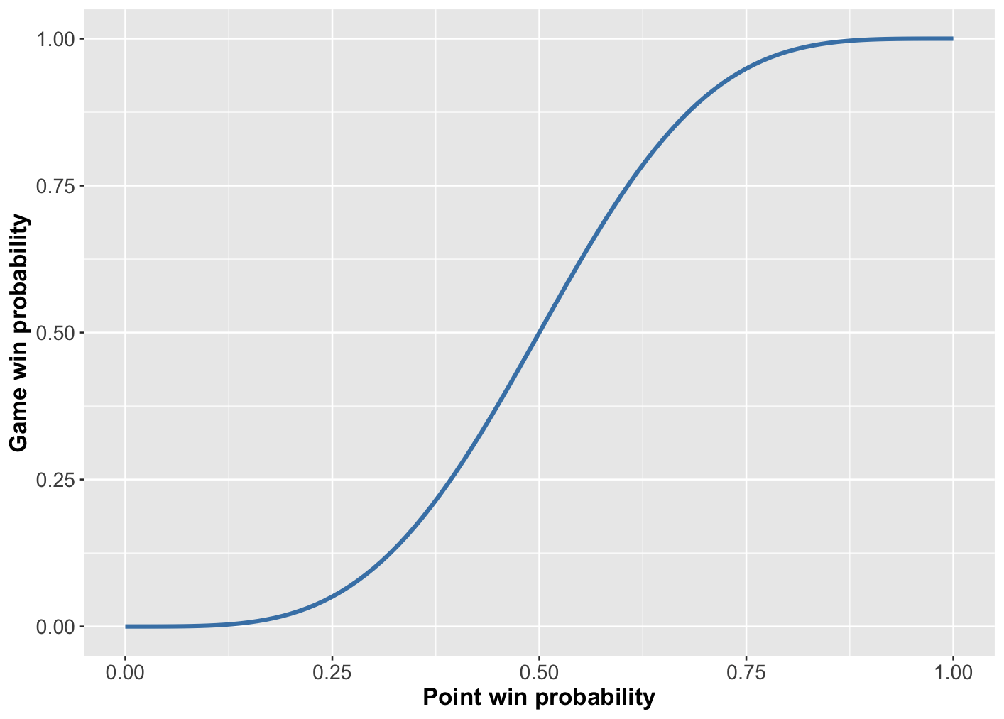
Figure 1: Probability of winning a game as a function of the probability of winning a point on serve.
Figure 1 shows the probability of the server winning a game as a function of their probability of winning any point on serve. As you’d expect, if the probability of the server winning a point is 0.5 – so each player is equally likely to win any point – then the probability of either player winning the game is 0.5. The serving player usually has an advantage though, so the point win probability for the server is usually greater than 0.5, even in games where the weaker player overall is serving. So, we’re mostly interested in the right-hand half of this figure.
A notable feature of Figure 1 is that game win probabilities grow much quicker than point win probabilities. For example, look at the figure at the point where the server has a 0.75 chance of winning a point. Their chance of winning the game is then around 0.95. That’s because although they’ve got a 25% chance of losing any point, the scoring rules of tennis mean it’s unlikely they lose a combination of points that results in them losing the game – the chance of that happening is only around 5%. So, the scoring rules ensure that a slight advantage in winning a point is magnified to a larger probability for winning a game.
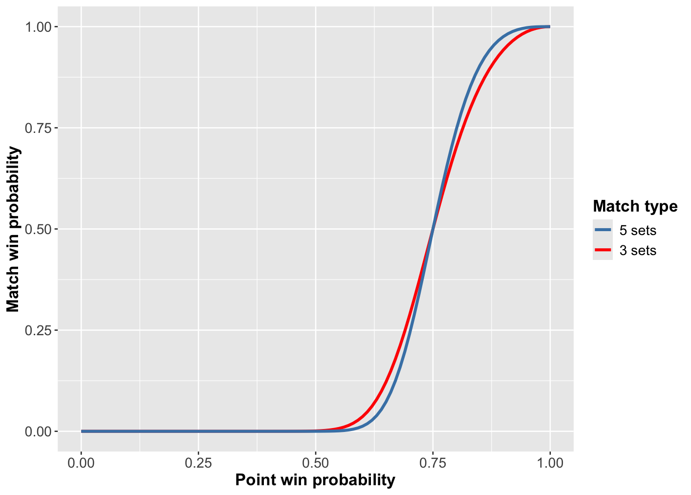
Figure 2: Match win probability as a function of point win probability on serve when the opponent’s point win probability on serve is 0.75
Similar techniques can be used to calculate the probability of either player winning a set or a match, though this also depends on the number of sets in a match – conventionally 3 or 5 – and the tiebreak rules. As an example, Figure 2 shows the probability of a player winning either a 3 or 5 set match, with standard tiebreak rules, as a function of their point win probability on serve when the opponent’s win probability on serve is 0.75.
- Naturally, as a player’s point win probability increases, so does their match win probability;
- When the player’s win probability on serve matches that of their opponent, at 0.75, the match win probability for either player is 0.5;
- The curves are steeper than the previous figure since a small change in point win probability on serve will lead to a bigger change in match win probability than the change in game win probability.
- Similarly, the curve for a 5-set match is steeper than for a 3-set match. Both these phenomena are due to the fact that the more points are played, the more likely it is that a player’s superiority will overcome the possibility of them losing by chance.
Now, we can return to the Isner-Mahut game and address the question: what was the probability of a final set score of 70-68? We’ll make things a bit easier by assuming each player had the same win probability p for a point on serve. This might seem a bit unrealistic as Isner was the number 23 seed, while Mahut was an unseeded qualifier. However, a detailed look at the numbers for the match shows that Isner and Mahut won 76.2% and 78.7% of points on serve respectively, so it’s not unreasonable to assume that each had a probability of around 0.775 of winning a point on serve.
For the final set to reach a score of 70-68, three things had to occur. First, the set had to reach the score of 6-6. Second, having reached that score, there had to be 62 further pairs of games in which the players shared the wins, so that the set score reached 68-68 without either player having had a two-game advantage at any stage. Finally, with the score at 68-68, one of the players had to win two consecutive games to take the set at 70-68.
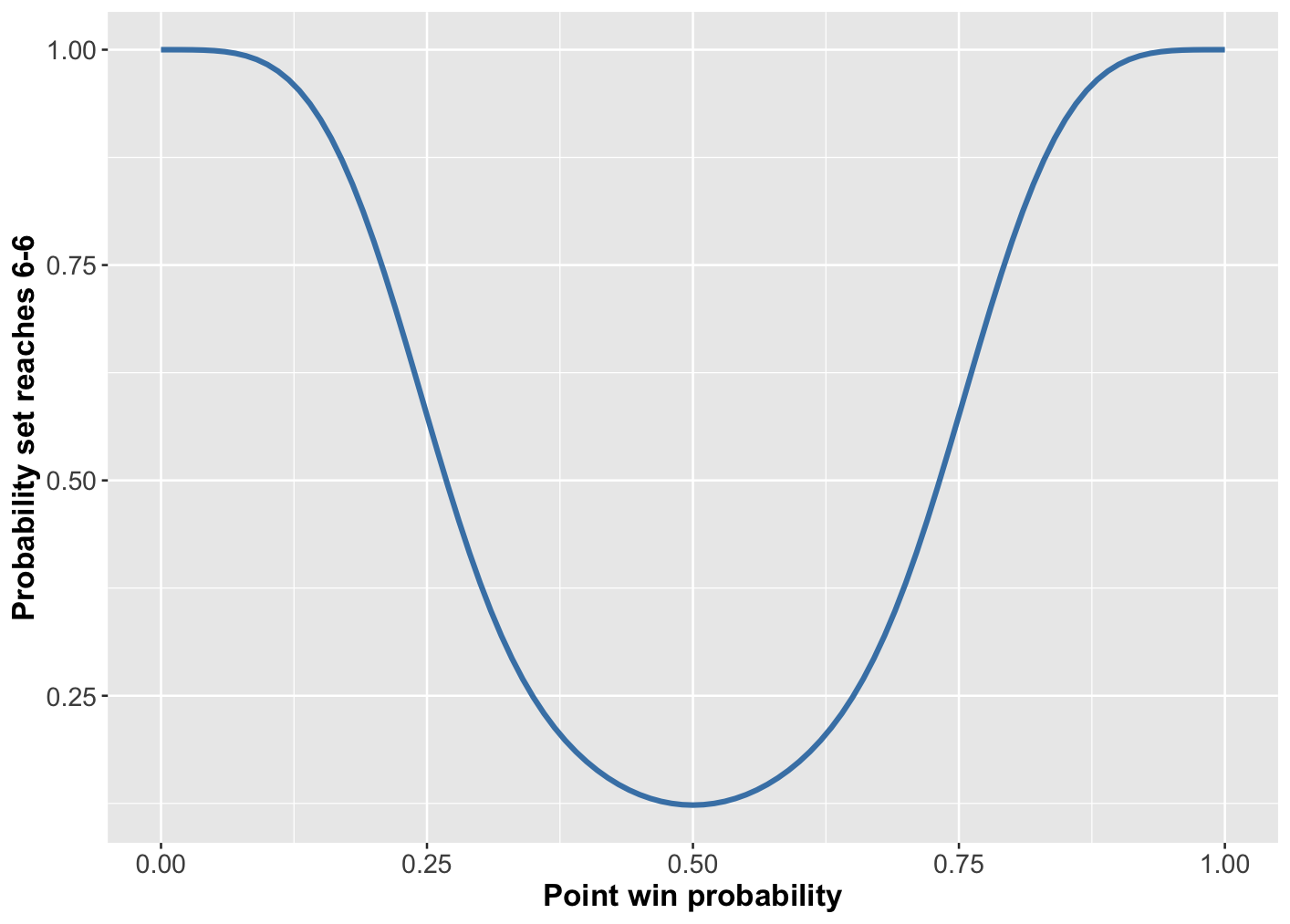
Figure 3: probability that a set reaches 6 games all as a function of the probability that either player wins a point on serve (assumed equal for both players).
Taking these things in turn, Figure 3 shows the probability of a set reaching 6-6 as a function of p, the probability of either player winning a point on serve. With p = 0.775, this takes a value around 0.682.
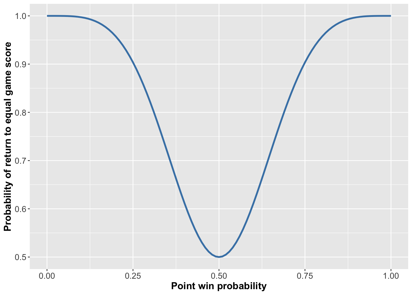
Figure 4: Probability final set returns to equal game score given current equal games score as a function of point win probability on serve (assumed equal for both players)
Once a score of 6-all is reached, every time the set is level in games, the probability it returns to being level after 2 further games is shown in Figure 4 as a function of p. With p = 0.775 this takes a value around 0.934. So, the probability of this occurring 62 times consecutively to reach an overall game score of 68-68 is 0.934 multiplied by itself 62 times.
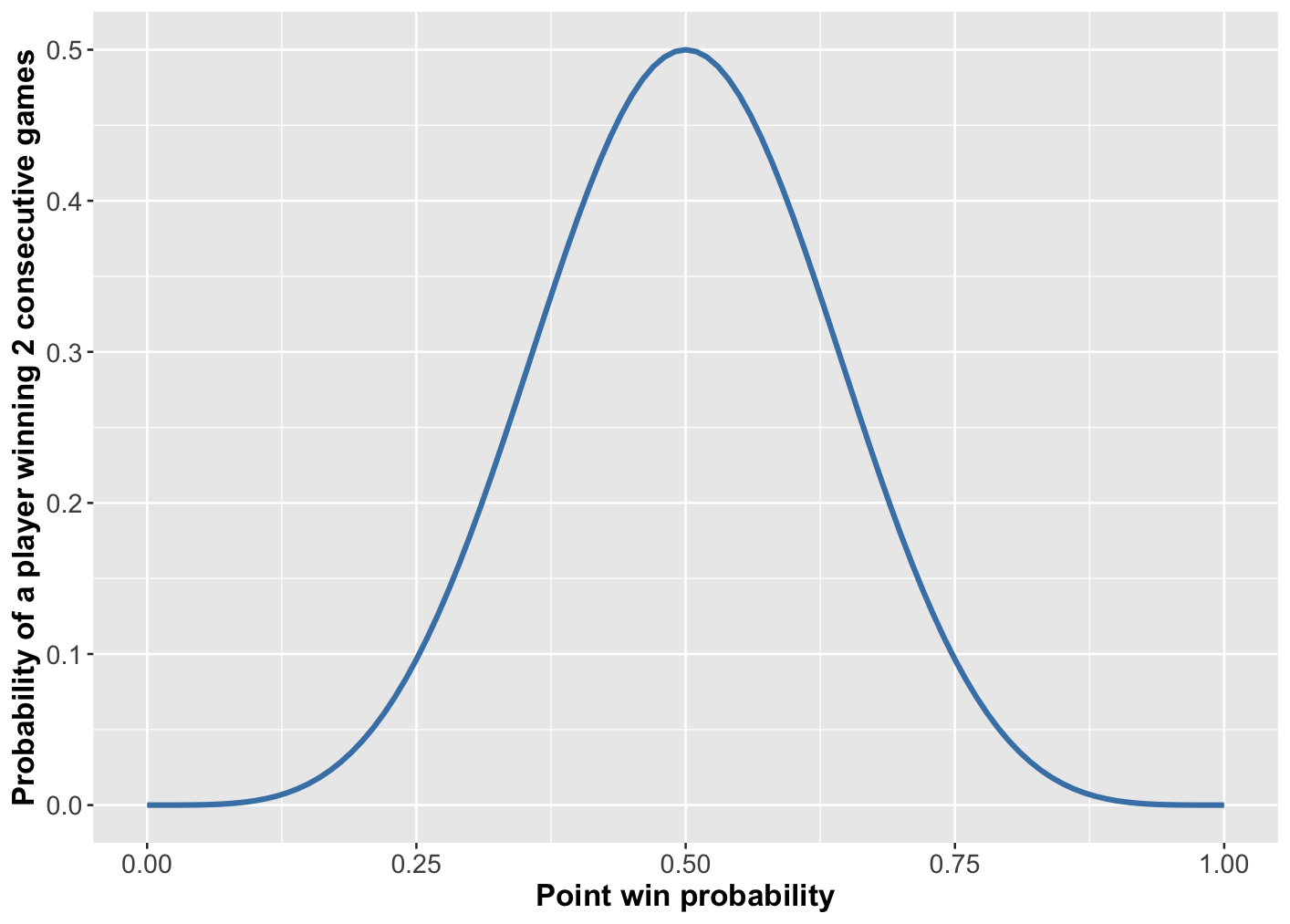
Figure 5: Probability of either player winning 2 consecutive games as a function of the point win probability on serve (assumed equal for each player).
Finally, we need one of the players to win 2 consecutive games, one on serve, one against serve. This is shown as a function of p in Figure 5. With p = 0.775 this is around 0.066.
Finally, putting everything together, this whole sequence of events leading to a final set score of 70-68 is
$ 0.683 \times 0.934^{62} \times 0.066 = 0.00065$
or roughly two-in-three-thousand.
So, given that the match got to the fifth set, subject to the independence assumption and based on the further assumption that each player would win a point on serve with probability 0.775, there was a two-in-three-thousand chance that the final set would finish 70-68.
How reasonable are the assumptions? They’re not perfect. It’s unlikely that a player’s point win probability stays constant throughout a match. For example, some players might be known to start slowly; others might be stronger on the more important points.
The assumption of independence is also likely to be false. If a player loses several points in a row, this is likely to be indicative of a loss of rhythm, in which case they are more likely to lose subsequent points.
Nevertheless, the calculation made under the assumptions of constant win probabilities and independence is likely to be reasonable as a kind of ‘ball-park’ figure. That being so, although two-in-three-thousand is a small probability, it’s perhaps not as small as one might have guessed. Certainly, my guess would have been much smaller. The reason it’s not smaller is that this match was characterised by dominance on serve from both players. Isner, in particular, was well-known to be a very strong server. By contrast, his ground strokes were relatively weak, meaning that an accurate – though not necessarily powerful – server like Mahut, would also win a high percentage of serves. Indeed, both players hit more than 100 aces in the match. This dominance of wins on service points from both players led to a situation where break points were both rare and rarely taken when they did occur, and the final set got stuck in a long sequence of games held to serve.
For comparison, the men’s final in 2010 was between Nadal and Berdych. This match was more one sided, with Nadal winning 73% of points on serve and Berdych 67%, and although it was completed in 3 sets, we can repeat the above calculation for the probability of an imaginary 5th set concluding with a game score of 70-68. To keep things simple, we’ll again assume that the two players were equally strong on serve, averaging the win proportions on serve to get p = 0.695. Repeating the previous calculation with this value of p leads to a probability of around one in 6.1 million for a final set score equal to 70-68 is . So with less dominant service games, the chance of reaching a set score as extreme as 70-68 is very much more remote, confirming that the outcome of the Isnet-Mahut match was really only plausible because of the playing characteristics of those players.
Finally, as a service to anyone who would prefer to have the story of the Isner-Mahut match provided in the form of a musical cappella rather than Statistics, please feel free to listen to this: