In a previous post I discussed a problem that Freddy had written to me about. The problem was a simplified version of an issue sent to him by friend, connected with a genetic algorithm for optimisation. Simply stated: you start with £100. You toss a coin and if it comes up tails you lose 25% of your current money, otherwise you gain 25%. You play this game over and over, always increasing or increasing your current money by 25% on the basis of a coin toss. The issue is how much money you expect to have, on average, after 1000 rounds of this game.
As I explained in the original post, Freddy’s intuition was that the average should stay the same at each round. So even after 1000 (or more) rounds, you’d have an average of £100. But when Freddy simulated the process, he always got an amount close to £0, and so concluded his intuition must be wrong.
A couple of you wrote to give your own interpretations of this apparent conflict, and I’m really grateful for your participation. As it turns out, Freddy’s intuition was spot on, and his argument was pretty much a perfect mathematical proof. Let me make the argument just a little bit more precise.
Suppose after n rounds the amount of money you have is M. Then after n+1 rounds you will have (3/4)M if you get a Head and (5/4)M if you get a Tail. Since each of these outcomes is equally probable, the average amount of money after n+1 rounds is
\frac{ (3/4)M + (5/4)M}{2}= MIn other words, exactly as Freddy had suggested, the average amount of money doesn’t change from one round to the next. And since I started with £100, this will be the average amount of money after 1 round, 2 rounds and all the way through to 1000 rounds.
But if Freddy’s intuition was correct, the simulations must have been wrong.
Well, no. I checked Freddy’s code – a world first! – and it was perfect. Moreover, my own implementation displayed the same features as Freddy’s, as shown in the previous post: every simulation has the amount of money decreasing to zero long before 1000 rounds have been completed.
So what explains this contradiction between what we can prove theoretically and what we see in practice?
The following picture shows histograms of the money remaining after a certain number of rounds for each of 100,000 simulations. In the previous post I showed the individual graphs of just 16 simulations of the game; here we’re looking at a summary of 100,000 simulated games.
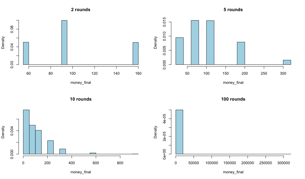
For example, after 2 rounds, there are only 3 possible outcomes: £56.25, £93.75 and £156.25. You might like to check why that should be so. Of these, £93.75 occurred most often in the simulations, while the other two occurred more or less equally often. You might also like to think why that should be so. Anyway, looking at the values, it seems plausible that the average is around £100, and indeed the actual average from the simulations is very close to that value. Not exact, because of random variation, but very close indeed.
After 5 rounds there are more possible outcomes, but you can still easily convince yourself that the average is £100, which it is. But once we get to 10 rounds, it starts to get more difficult. There’s a tendency for most of the simulated runs to give a value that’s less than £100, but then there are relatively few observations that are quite a bit bigger than £100. Indeed, you can just about see that there is one or more value close to £1000 or so. What’s happening is that the simulated values are becoming much more asymmetric as the number of rounds increases. Most of the results will end up below £100 – though still positive, of course – but a few will end up being much bigger than £100. And the average remains at £100, exactly as the theory says it must.
After 100 rounds, things are becoming much more extreme. Most of the simulated results end up close to zero, but one simulation (in this case) gave a value of around £300,000. And again, once the values are averaged, the answer is very close to £100.
But how does this explain what we saw in the previous post? All of the simulations I showed, and all of those that Freddy looked at, and those his friend obtained, showed the amount of money left being essentially zero after 1000 rounds. Well, the histogram of results after 1000 rounds is a much, much more extreme case of the one shown above for 100 rounds. Almost all of the probability is very, very close to zero. But there’s a very small amount of probability spread out up to an extremely large value indeed, such that the overall average remains £100. So almost every time I do a simulation of the game, the amount of money I have is very, very close to zero. But very, very, very occasionally, I would simulate a game whose result was a huge amount of money, such that it would balance out all of those almost-zero results and give me an answer close to £100. But, such an event is so rare, it might take billions of billions of simulations to get it. And we certainly didn’t get it in the 16 simulated games that I showed in the previous post.
So, there is no contradiction at all between the theory and the simulations. It’s simply that when the number of rounds is very large, the very large results which could occur after 1000 rounds, and which ensure that the average balances out to £100, occur with such low probability that we are unlikely to simulate enough games to see them. We therefore see only the much more frequent games with low winnings, and calculate an average which underestimates the true value of £100.
There are a number of messages to be drawn from this story:
- Statistical problems often arise in the most surprising places.
- The strategy of problem simplification, solution through intuition, and verification through experimental results is a very useful one.
- Simulation is a great way to test models and hypotheses, but it has to be done with extreme care.
- And if there’s disagreement between your intuition and experimental results, it doesn’t necessarily imply either is wrong. It may be that the experimental process has complicated features that make results unreliable, even with a large number of simulations.
Thanks again to Freddy for the original problem and the discussions it led to.
To be really precise, there’s a bit of sleight-of-hand in the mathematical argument above. After the first round my expected – rather than actual – amount of money is £100. What I showed above is that the average money I have after any round is equal to the actual amount of money I have at the start of that round. But that’s not quite the same thing as showing it’s equal to the average amount of money I have at the start of the round.
But there’s a famous result in probability – sometimes called the law of iterated expectations – which lets me replace this actual amount at the start of the second round with the average amount, and the result stays the same. You can skip this if you’re not interested, but let me show you how it works.
At the start of the first round I have £100.
Because of the rules of the game, at the end of this round I’ll have either £75 or £125, each with probability 1/2.
In the first case, after the second round, I’ll end up with either £56.25 or £93.75, each with probability 1/2. And the average of these is £75.
In the second case, after the second round, I’ll end up with either £93.75 or £125.75, each with probability 1/2. And the average of these is £125.
And if I average these averages I get £100. This is the law of iterated expectations at work. I’d get exactly the same answer if I averaged the four possible 2-round outcomes: £56.25, £93.75 (twice) and £125.75.
Check:
\frac{56.25 + 93.75 + 93.75 + 125.75}{4} = 100
So, my average after the second round is equal to the average after the first which was equal to the initial £100.
The same argument also applies at any round: the average is equal to the average of the previous round. Which in turn was equal to the average of the previous round. And so on, telescoping all the way back to the initial value of £100.
So, despite the sleight-of-hand, the result is actually true, and this is precisely what Freddy had hypothesised. As explained above, his only ‘mistake’ was to observe that a small number of simulations suggested a quite different behaviour, and to assume that this meant his mathematical reasoning was wrong.